Discussion about an ongoing work.
Introduction
Experimentation about a method for online learning and controlling system with uncertainty.
The aim of this work is to take advantage of smart exploration algorithms in order to more efficiently build a control policy based on the Quasimetric method.
For details about the Quasimetric method see http://www.plosone.org/article/info%3Adoi%2F10.1371%2Fjournal.pone.0083411
The problem here is to control an (uncertain) dynamical system modelled as a Markovian Decision Process (MDP) with the transition probability P(X^{t+1}|X^{t},U^{t}), with X the state and U the action.
To do so we use the Quasimetric method on which we added learning capabilities, i.e. learning P(X^{t+1}|X^{t},U^{t}) with a Laplace succession law (ask if you want more details).
This method allows us to compute a policy P(U|X) for reach a given goal.
The problem is that initially the dynamical model contains no information and the policy is uniform, thus random.
Here we are interested in finding an efficient way to explore the state space in order to learn the model and thus the control policy.
-
A first way to explore is obviously to continuously apply a random action (random motor).
The problem is that this procedure may be quite inefficient to reach difficult state space regions and moreover it doesn’t use the learned model. -
Another possibility is to try to explore the state space more uniformly by choosing goals in the state space (randomly) and then use the policy from the learned model to reach it (random goal).
The problem here is that the state space may not be uniformly interesting to explore. -
Finally, we can try to chose goals in the state space using a curiosity-based paradigm. This kind of methods allows to concentrate more on state space regions where more progresses are made (progress tracking).
Experiment
A simple test was done with a simulated "noisy’’ inverted pendulum. The associated state space was the pendulum position (angular) and its velocity (2D state space). The control space is the torque of the pendulum (1D action space). The later was chosen to be limited so that the state space can only be explored by using the dynamics of the pendulum, i.e. balancing several times.
In the test procedure we start without any knowledge (uniform probabilities) and the aim is to simultaneously explore and construct a model and a Quasimetric. Then, the Quasimetric can be used to compute a policy to reach a chosen goal.
An experiment epoch is done by simulating the pendulum for a maximum of 300 timesteps (until the goal is reached), starting from the low equilibrium position. Depending on the tested method (random motor, random goal or discrete progress), for each epoch the policy is respectively random, based on a randomly chosen goal or based on a discrete progress tracking chosen goal.
- In the random motor method, we simply apply a random motor command continuously and learn the model.
- In the random goal method, we randomly chose a goal and then apply the current policy to reach that goal (while learning the model).
- In the Discrete progress method, we chose the goal according to the competence progress of the system, and then apply the current policy to reach that goal (while learning).
For each goal we track the competence progress in the recent trials to reach that goal (see https://hal.inria.fr/hal-00860641 ask for more details).
Then for each chosen goal a policy is computed based on the current model and Quasimetric. A complete run is composed of 10000 successive epochs.
Preliminary results
Comparing policies
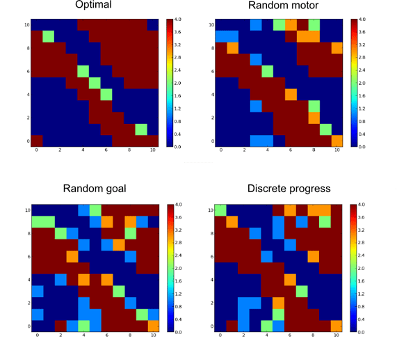
Here are examples of obtained policies toward a specific goal (the vertical unstable equilibrium) for each method after 10000 epochs compared with the optimal policy (computed with Value Iteration).
Angular position in x and angular velocity in y (vertical equilibrium position with zero velocity in the center). Color code represents the action (most probable action).
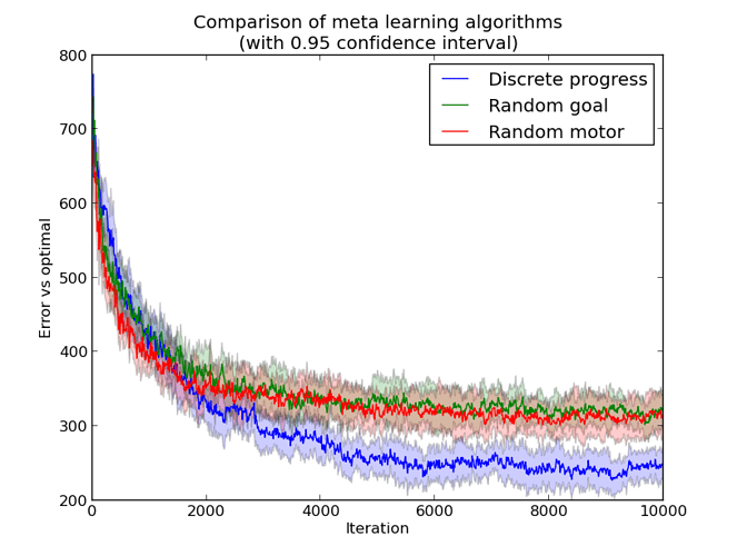
If we look at the evolution of these policies through iteration (square error compared to the optimal) we can see a slight improvement after a while, using the Discrete Progress:
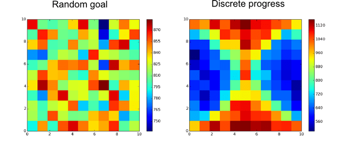
In fact, as expected, if we look at the chosen goals for the Discrete Progress method (compared to random goal) we can see that the “easy” part of the state space if less explored than the “difficult” one:
Questions/Remarks
It is not clear if one method is really better than another at improving the overall learning performance.
How to evaluate/compare the different exploration methods?
The error to the optimal is maybe not a good metric.
We tested the time to reach a goal and no clear differences appeared.


