Reproducibility in Machine Learning and Deep Reinforcement Learning in particular has become a serious issue in the recent years. Reproducing an RL paper can turn out to be much more complicated than you thought, see this blog post about lessons learned from reproducing a deep RL paper. Indeed, codebases are not always released and scientific papers often omit parts of the implementation tricks. Recently, Henderson et al. conducted a thorough investigation of various parameters causing this reproducibility crisis [Henderson et al., 2017]. They used trendy deep RL algorithms such as DDPG, ACKTR, TRPO and PPO with OpenAI Gym popular benchmarks such as Half-Cheetah, Hopper and Swimmer to study the effects of the codebase, the size of the networks, the activation function, the reward scaling or the random seeds. Among other results, they showed that different implementations of the same algorithm with the same set of hyperparameters led to drastically different results.
Perhaps the most surprising thing is this: running the same algorithm 10 times with the same hyper-parameters using 10 different random seeds and averaging performance over two splits of 5 seeds can lead to learning curves seemingly coming from different statistical distributions. Then, they present this table:
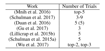
This table shows that all the deep RL papers reviewed by Henderson et al. use less than 5 seeds. Even worse, some papers actually report the average of the best performing runs! As demonstrated in Henderson et al., these methodologies can lead to claim that two algorithms performances are different when they are not. A solution to this problem is to use more random seeds, to average more different trials to obtain a more robust measure of your algorithm performance. OK, but how many more? Should I use 10, should I use 100 as in [Mania et al, 2018]? The answer is, of course, it depends.
If you read this blog, you must be in the following situation: you want to compare the performance of two algorithms to determine which one performs best in a given environment. Unfortunately, two runs of the same algorithm often yield different measures of performance. This might be due to various factors such as the seed of the random generators (called random seed or seed thereafter), the initial conditions of the agent, the stochasticity of the environment, etc.
Part of the statistical procedures described in this article are available on Github here. The article is available on ArXiv here.
Definition of the statistical problem
The performance of an algorithm can be modeled as a random variable X and running this algorithm in an environment results in a realization x. Repeating the procedure N times, you obtain a statistical sample x=(x^1, .., x^N). A random variable is usually characterized by its mean \mu and its standard deviation, noted \sigma. Of course, you do not know what are the values of \mu and \sigma. The only thing you can do is to compute their estimations \overline{x} and s:
where \overline{x} is called the empirical mean, and s is called the empirical standard deviation. The larger the sample size N, the more confidence you can be in the estimations.
Here, two algorithms with respective performances X_1 and X_2 are compared. If X_1 and X_2 follow normal distributions, the random variable describing their difference (X_{\text{diff}} = X_1-X_2) also follows a normal distribution with parameters {\sigma_{diff}=(\sigma_1^2+\sigma_2^2)^{1/2}} and \mu_{\text{diff}}=\mu_1-\mu_2. In this case, the estimator of the mean of X_{\text{diff}} is \overline{x}_{\text{diff}} = \overline{x}_1-\overline{x}_2 and the estimator of {\sigma_{\text{diff}}} is {s_{\text{diff}}=\sqrt{s_1^2+s_2^2}}. The effect size \epsilon can be defined as the difference between the mean performances of both algorithms: {\epsilon = \mu_1-\mu_2}.
Testing for a difference between the performances of two algorithms (\mu_1 and \mu_2) is mathematically equivalent to testing a difference between their difference \mu_{\text{diff}} and 0. The second point of view is considered from now on. We draw a sample x_{\text{diff}} from X_{\text{diff}} by subtracting two samples x_1 and x_2 obtained from X_1 and X_2.
Example 1
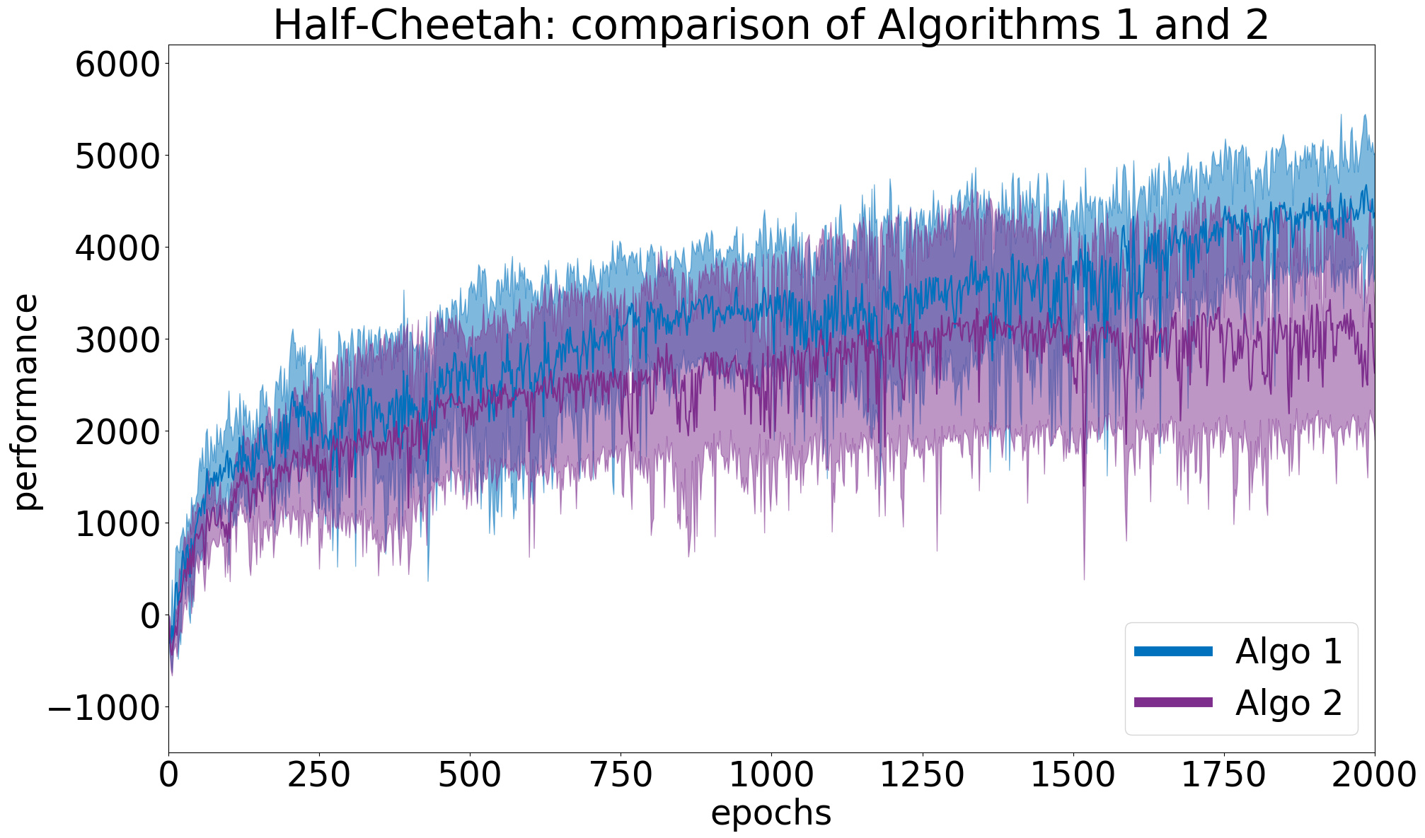
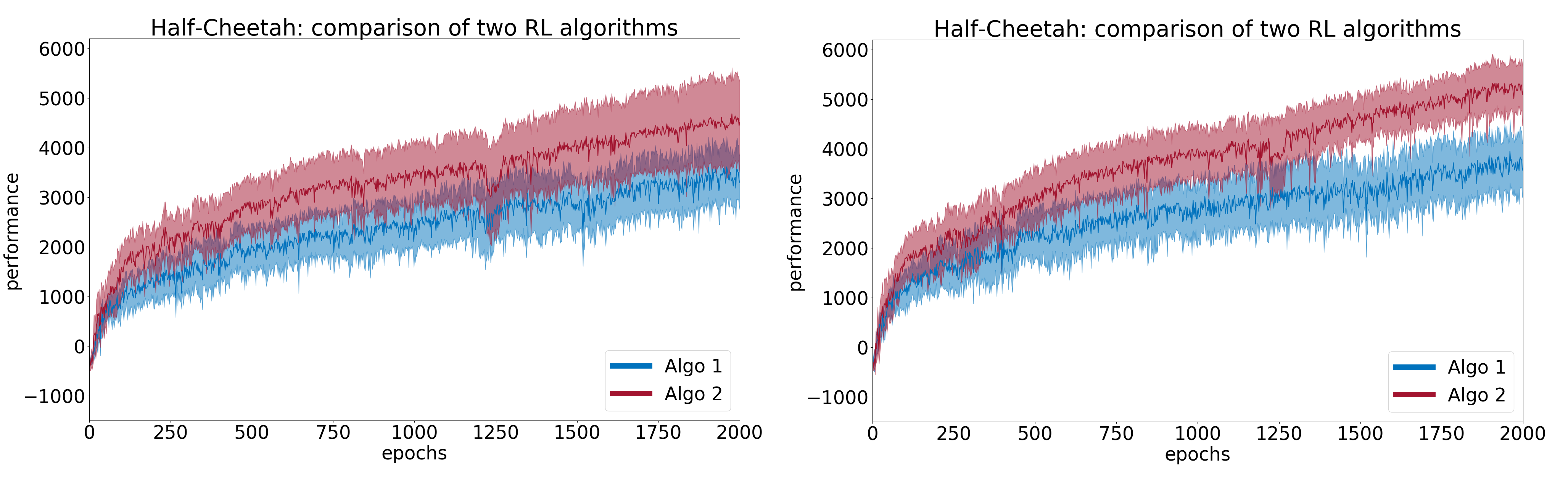
To illustrate the concepts developed in this article, let us take two algorithms (Algo 1 and Algo 2) and compare them on the Half-Cheetah environment from the OpenAI Gym framework. The actual algorithms used are not so important here, and will be revealed later. First, we run a preliminary study with N=5 random seeds for each and plot the results in Figure 2. This figure shows the average learning curves, with the 95\% confidence interval. Each point of a learning curve is the average cumulated reward over 10 evaluation episodes. The measure of performance of an algorithm is the average performance over the last 10 points (i.e. last 100 evaluation episodes). From the figure, it seems that Algo1 performs better than Algo2. Moreover, the confidence intervals do not overlap much at the end. Of course, we need to run statistical tests before drawing any conclusion.
Comparing performances with a difference test
In a difference test, statisticians define the null hypothesis H_0 and the alternate hypothesis H_a. H_0 assumes no difference whereas H_a assumes one:
- H_0: \mu_{\text{diff}} = 0
- H_a: \mu_{\text{diff}} \neq 0
These hypothesis refers to the two-tail case. When you have an a-priori on which algorithm performs best, (let us say Algo1), you can use the one-tail version:
- H_0: \mu_{\text{diff}} \leq 0
- H_a: \mu_{\text{diff}} > 0
At first, a statistical test always assumes the null hypothesis. Once a sample x_{\text{diff}} is collected from X_{\text{diff}}, you can estimate the probability p (called p-value) of observing data as extreme, under the null hypothesis assumption. By extreme, one means far from the null hypothesis (\overline{x}_{\text{diff}} far from 0). The p-value answers the following question: how probable is it to observe this sample or a more extreme one, given that there is no true difference in the performances of both algorithms? Mathematically, we can write it this way for the one-tail case:
and this way for the two-tail case:
When this probability becomes really low, it means that it is highly improbable that two algorithms with no performance difference produced the collected sample x_{\text{diff}}. A difference is called significant at significance level \alpha when the p-value is lower than \alpha in the one-tail case, and lower than \alpha/2 in the two tail case (to account for the two-sided test). Usually \alpha is set to 0.05 or lower. In this case, the low probability to observe the collected sample under hypothesis H_0 results in its rejection. Note that a significance level \alpha=0.05 still results in 1 chance out of 20 to claim a false positive, to claim that there is a true difference when there is not.
Another way to see this, is to consider confidence intervals. Two kinds of confidence intervals can be computed:
- CI_1: The 100\cdot(1-\alpha)\hspace{3pt}\% confidence interval for the mean of the difference \mu_{\text{diff}} given a sample x_{\text{diff}} characterized by \overline{x}_{\text{diff}} and s_{\text{diff}}.
- CI_2: The 100\cdot(1-\alpha)\hspace{3pt}\% confidence interval for any realization of X_{\text{diff}} under H_0 (assuming \mu_{\text{diff}}=0).
Having CI_2 that does not include \overline{x}_{\text{diff}} is mathematically equivalent to a p-value below \alpha. In both cases, it means there is less than 100\cdot\alpha\% chance that \mu_{\text{diff}}=0 under H_0. When CI_1 does not include 0, we are also 100\cdot(1-\alpha)\hspace{3pt}\% confident that \mu\neq0, without assuming H_0. Proving one of these things leads to conclude that the difference is significant at level \alpha.
Two types of errors can be made in statistics:
- The type-I error rejects H_0 when it is true, also called false positive. This corresponds to claiming the superiority of an algorithm over another when there is no true difference. Note that we call both the significance level and the probability of type-I error \alpha because they both refer to the same concept. Choosing a significance level of \alpha enforces a probability of type-I error \alpha, under the assumptions of the statistical test.
- The type-II error fails to reject H_0 when it is false, also called false negative. This corresponds to missing the opportunity to publish an article when there was actually something to be found.
Important:
- In the two-tail case, the null hypothesis H_0 is \mu_{\text{diff}}=0. The alternative hypothesis H_a is \mu_{\text{diff}}\neq0.
- p{\normalsize \text{-value}} = P(X_{\text{diff}}\geq \overline{x}_{\text{diff}} \hspace{2pt} |\hspace{2pt} H_0).
- A difference is said statistically significant when a statistical test passed. One can reject the null hypothesis when 1) p-value <\alpha; 2) CI_1 does not contain 0; 3) CI_2 does not contain \overline{x}_{\text{diff}}.
- statistically significant does not refer to the absolute truth. Two types of error can occur. Type-I error rejects H_0 when it is true. Type-II error fails to reject H_0 when it is false.
Select the appropriate statistical test
You must decide which statistical tests to use in order to assess whether the performance difference is significant or not. As recommended in [Henderson et al., 2017], the two-sample t-test and the bootstrap confidence interval test can be used for this purpose. Henderson et al. also advised for the Kolmogorov-Smirnov test, which tests if two samples comes from the same distribution. This test should not be used to compare RL algorithms because it is unable to prove any order relation.
T-test and Welch’s t-test
We want to test the hypothesis that two populations have equal means (null hypothesis H_0). A 2-sample t-test can be used when the variances of both populations (both algorithms) are assumed equal. However, this assumption rarely holds when comparing two different algorithms (e.g. DDPG vs TRPO). In this case, an adaptation of the 2-sample t-test for unequal variances called Welch’s t-test should be used. T-tests make a few assumptions:
- The scale of data measurements must be continuous and ordinal (can be ranked). This is the case in RL.
- Data is obtained by collecting a representative sample from the population. This seem reasonable in RL.
- Measurements are independent from one another. This seems reasonable in RL.
- Data is normally-distributed, or at least bell-shaped. The normal law being a mathematical concept involving infinity, nothing is ever perfectly normally distributed. Moreover, measurements of algorithm performances might follow multi-modal distributions.
Under these assumptions, one can compute the t-statistic t and the degree of freedom \nu for the Welch’s t-test as estimated by the Welch–Satterthwaite equation, such as:
with x_{\text{diff}} = x_1-x_2; s_1, s_2 the empirical standard deviations of the two samples, and N the sample size (same for both algorithms). The t-statistics are assumed to follow a t-distribution, which is bell-shaped and whose width depends on the degree of freedom. The higher this degree, the thinner the distribution.
Figure 3 helps making sense of these concepts. It represents the distribution of the t-statistics corresponding to X_{\text{diff}}, under H_0 (left distribution) and under H_a (right distribution). H_0 assumes \mu_{\text{diff}}=0, the distribution is therefore centered on 0. H_a assumes a (positive) difference \mu_{\text{diff}}=\epsilon, the distribution is therefore shifted by the t-value corresponding to \epsilon, t_\epsilon. Note that we consider the one-tail case here, and test for a positive difference.
A t-distribution is defined by its probability density functionT_{distrib}^{\nu}(\tau) (left curve in Figure 3, which is parameterized by \nu. The cumulative distribution function CDF_{H_0}(t) is the function evaluating the area under T_{distrib}^{\nu}(t) from \tau=-\infty to \tau=t. This allows to write:
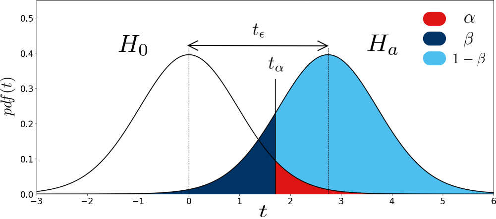
In Figure 3, t_\alpha represents the critical t-value to satisfy the significance level \alpha in the one-tail case. When t=t_\alpha, p-value =\alpha. When t>t_\alpha, the p-value is lower than \alpha and the test rejects H_0. On the other hand, when t is lower than t_\alpha, the p-value is superior to \alpha and the test fails to reject H_0. As can be seen in the figure, setting the threshold at t_\alpha might also cause an error of type-II. The rate of this error (\beta) is represented by the dark blue area: under the hypothesis of a true difference \epsilon (under H_a, right distribution), we fail to reject H_0 when t is inferior to t_\alpha. \beta can therefore be computed mathematically using the CDF:
Using the translation properties of integrals, we can rewrite \beta as:
The procedure to run a Welch’s t-test given two samples (x_1, x_2) is:
- Computing the degree of freedom \nu and the t-statistic t based on s_1, s_2, N and \overline{x}_{\text{diff}}.
- Looking up the t_\alpha value for the degree of freedom \nu in a t-table or by evaluating the inverse of the CDF function in \alpha.
- Compare the t-statistic to t_\alpha. The difference is said statistically significant (H_0 rejected) at level \alpha when t\geq t_\alpha.
Note that t<t_\alpha does not mean there is no difference between the performances of both algorithms. It only means there is not enough evidence to prove its existence with 100 \cdot (1-\alpha)\% confidence (it might be a type-II error). Noise might hinder the ability of the test to detect the difference. In this case, increasing the sample size N could help uncover the difference.
Selecting the significance level \alpha of the t-test enforces the probability of type-I error to \alpha. However, Figure 3 shows that decreasing this probability boils down to increasing t_\alpha, which in turn increases the probability of type-II error \beta. One can decrease \beta while keeping \alpha constant by increasing the sample size N. This way, the estimation \overline{x}_{\text{diff}} of \overline{\mu}_{\text{diff}} gets more accurate, which translates in thinner distributions in the figure, resulting in a smaller \beta. The next section gives standard guidelines to select N so as to meet requirements for both \alpha and \beta.
Bootstrapped confidence intervals
Bootstrapped confidence interval is a method that does not make any assumption on the distributions of performance differences. It estimates the confidence intervals by re-sampling among the samples actually collected and by computing the mean of each generated sample.
Given the true mean \mu and standard deviation \sigma of a normal distribution, a simple formula gives the 95\% confidence interval. But here, we consider an unknown distribution F (the distribution of performances for a given algorithm). As we saw above, the empirical mean \overline{x} is an unbiased estimate of its true mean, but how do we compute a confidence interval? One solution is to use the bootstrap principle.
Let us say we have a sample x_1, x_2, .., x_N of measures (performance measures in our case), where N is the sample size. The empirical bootstrap sample is obtained by sampling with replacement inside the original sample. This bootstrap sample is noted x^*_1, x^*_2, …, x^*_N and has the same number of measurements N. The bootstrap principle then says that, for any statistics u computed on the original sample and u^* computed on the bootstrap sample, variations in u are well approximated by variations in u^*. More explanations and justifications can be found in this document from MIT. You can therefore approximate variations of the empirical mean (let’s say its range), by variations of the bootstrapped samples.
The computation would look like this:
- Generate B bootstrap samples of size N from the original sample x_1 of Algo1 and B samples from from the original sample x_2 of Algo2.
- Compute the empirical mean for each sample: \mu^1_1, \mu^2_1, ..., \mu^B_1 and \mu^1_2, \mu^2_2, ..., \mu^B_2
- Compute the differences \mu_{\text{diff}}^{1:B} = \mu_1^{1:B}-\mu_2^{1:B}
- Compute the bootstrapped confidence interval at 100\cdot(1-\alpha)\%. This is basically the range between the 100 \cdot\alpha/2 and 100\cdot(1-\alpha)/2 percentiles of the vector \mu_{\text{diff}}^{1:B} (e.g. for \alpha=0.05, the range between the 2.5^{th} and the 97.5^{th} percentiles).
The number of bootstrap samples B should be chosen large (e.g. >1000). If the confidence interval bounds does not contain 0, it means that you are confident at 100 \cdot (1-\alpha)% that the difference is either positive (both bounds positive) or negative (both bounds negative). You just found a statistically significant difference between the performances of your two algorithms. You can find a nice implementation of this here.
Example 1 (continued)
Here, the type-I error requirement is set to \alpha=0.05. Running the Welch’s t-test and the bootstrap confidence interval test with two samples (x_1,x_2) of 5 seeds each leads to a p-value of 0.031 and a bootstrap confidence interval such that P\big(\mu_{\text{diff}} \in [259, 1564]\big) = 0.05. Since the p-value is below the significance level \alpha and the CI_1 confidence interval does not include 0, both test passed. This means both tests found a significant difference between the performances of Algo1 and Algo2 with a 95\% confidence. There should have been only 5\% chance to conclude a significant difference if it did not exist.
In fact, we did encounter a type-I error. I know that for sure because:
They are both the canonical implementation of DDPG [Lillicrap et al., 2015]. The codebase can be found on this repository. This means that H_0 was the true hypothesis, there is no possible difference in the true means of the two algorithms. Our first conclusion was wrong, we committed a type-I error, rejecting H_0 when it was true. In our case, we selected the two tests so as to set the type-I error probability \alpha to 5\%. However, statistical tests often make assumptions, which results in wrong estimations of the probability of the type-I error. We will see in the last section that the false positive rate was strongly under-evaluated.
Important:
- T-tests assume t-distributions of the t-values. Under some assumptions, they can compute analytically the p-value and the confidence interval CI_2 at level \alpha.
- The Welch’s t-test does not assume both algorithms have equal variances but the t-test does.
- The bootstrapped confidence interval test does not make assumptions on the performance distribution and estimates empirically the confidence interval CI_1 at level \alpha.
- Selecting a test with a significance level \alpha enforces a type-I error \alpha when the assumptions of the test are verified.
The theory: power analysis for the choice of the sample size
We saw that \alpha was enforced by the choice of the significance level in the test implementation. The second type of error \beta must now be estimated. \beta is the probability to fail to reject H_0 when H_a is true. When the effect size \epsilon and the probability of type-I error \alpha are kept constant, \beta is a function of the sample size N. Choosing N so as to meet requirements on \beta is called statistical power analysis. It answers the question: what sample size do I need to have 1-\beta chance to detect an effect size \epsilon, using a test with significance level \alpha? The next paragraphs present guidelines to choose N in the context of a Welch’s t-test.
As we saw above, \beta can be analytically computed as:
where CDF_{H_0} is the cumulative distribution function of a t-distribution centered on 0, t_\alpha is the critical value for significance level \alpha and t_\epsilon is the t-value corresponding to an effect size \epsilon. In the end, \beta depends on \alpha, \epsilon, (s_1, s_2) the empirical standard deviations computed on two samples (x_1,x_2) and the sample size N.
Example 2
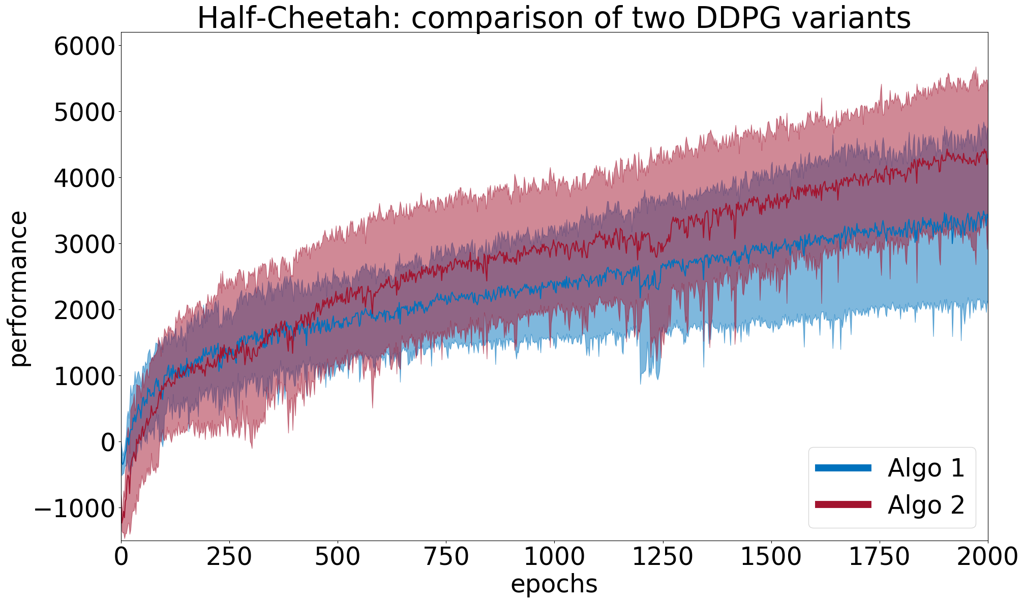
To illustrate, we compare two DDPG variants: one with action perturbations (Algo 1) [Lillicrap et al., 2015], the other with parameter perturbations (Algo 2) [Plappert et al., 2017]. Both algorithms are evaluated in the Half-Cheetah environment from the OpenAI Gym framework.
Step 1 - Running a pilot study
To compute \beta, we need estimates of the standard deviations of the two algorithms (s_1, s_2). In this step, the algorithms are run in the environment to gather two samples x_1 and x_2 of size n. From there, we can compute the empirical means (\overline{x}_1, \overline{x}_2) and standard deviations (s_1, s_2).
Example 2 (continued)
Here we run both algorithms with n=5. We find empirical means (\overline{x}_1, \overline{x}_2) = (3523, 4905) and empirical standard deviations (s_1, s_2) = (1341, 990) for Algo1 (blue) and Algo2 (red) respectively. From Figure 4, it seems there is a slight difference in the mean performances \overline{x}_{\text{diff}} =\overline{x}_2-\overline{x}_1 >0.
Running preliminary statistical tests at level \alpha=0.05 lead to a p-value of 0.1 for the Welch’s t-test, and a bootstrapped confidence interval of CI_1=[795, 2692] for the value of \overline{x}_{\text{diff}} = 1382. The Welch’s t-test does not reject H_0 (p-value >\alpha) but the bootstrap test does (0\not\in CI_1). One should compute \beta to estimate the chance that the Welch’s t-test missed an underlying performance difference (type-II error).
Step 2 - Choosing the sample size
Given a statistical test (Welch’s t-test), a significance level \alpha (e.g. \alpha=0.05) and empirical estimations of the standard deviations of Algo1 and Algo2 (s_1,s_2), one can compute \beta as a function of the sample size N and the effect size \epsilon one wants to be able to detect.
Example 2 (continued)
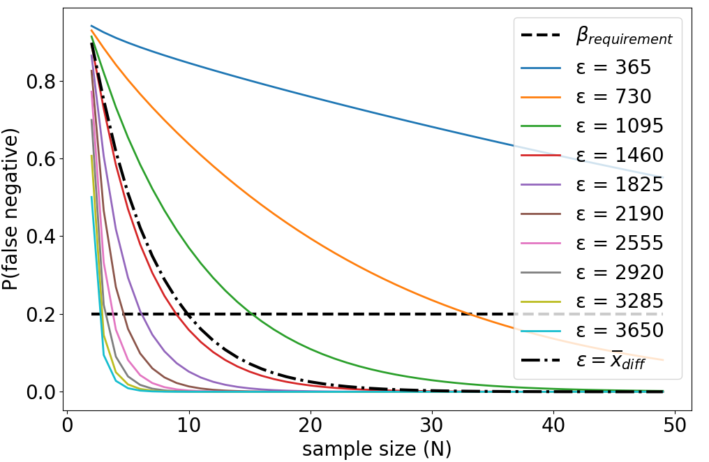
For N in [2,50] and \epsilon in [0.1,..,1]\times\overline{x}_1, we compute t_\alpha and \nu using the formulas given in Section \ref{sec:ttest}, as well as t_{\epsilon} for each \epsilon. Finally, we compute the corresponding probability of type-II error \beta using Equation~\ref{eq:beta}. Figure 5 shows the evolution of \beta as a function of N for the different \epsilon. Considering the semi-dashed black line for \epsilon=\overline{x}_{\text{diff}}=1382, we find \beta=0.51 for N=5: there is 51\% chance of making a type-II error when trying to detect an effect \epsilon=1382. To meet the requirement \beta=0.2, N should be increased to N=10 (\beta=0.19).
In our example, we find that N=10 was enough to be able to detect an effect size \epsilon=1382 with a Welch’s t-test, using significance level \alpha and using empirical estimations (s_1, s_2) = (1341, 990). However, let us keep in mind that these computations use various approximations (\nu, s_1, s_2) and make assumptions about the shape of the t-values distribution.
Step 3 - Running the statistical tests
Both algorithms should be run so as to obtain a sample x_{\text{diff}} of size N. The statistical tests can be applied.
Example 2 (continued)
Here, we take N=10 and run both the Welch’s t-test and the bootstrap test. We now find empirical means (\overline{x}_1, \overline{x}_2) = (3690, 5323) and empirical standard deviations (s_1, s_2) = (1086, 1454) for Algo1 and Algo2 respectively. Both tests rejected H_0, with a p-value of 0.0037 for the Welch’s t-test and a confidence interval for the difference \mu_{\text{diff}} \in [732,2612] for the bootstrap test. Both tests passed. In Figure 7, plots for N=5 and N=10 can be compared. With a larger number of seeds, the difference that was not found significant with N=5 is now more clearly visible. With a larger number of seeds, the estimate \overline{x}_{\text{diff}} is more robust, more evidence is available to support the claim that Algo2 outperforms Algo1, which translates to tighter confidence intervals represented in the figures.
\end{myex}
Important:
Given a sample size N, a minimum effect size to detect \epsilon and a requirement on type-I error \alpha the probability of type-II error \beta can be computed. This computation relies on the assumptions of the t-test.
The sample size N should be chosen so as to meet the requirements on \beta.
In practice: influence of deviations from assumptions
Under their respective assumptions, the t-test and bootstrap test enforce the probability of type-I error to the selected significance level \alpha. These assumptions should be carefully checked, if one wants to report the probability of errors accurately. First, we propose to compute an empirical evaluation of the type-I error based on experimental data, and show that: 1) the bootstrap test is sensitive to small sample sizes; 2) the t-test might slightly under-evaluate the type-I error for non-normal data. Second, we show that inaccuracies in the estimation of the empirical standard deviations s_1 and s_2 due to low sample size might lead to large errors in the computation of \beta, which in turn leads to under-estimate the sample size required for the experiment.
Empirical estimation of the type-I error
Remember, type-I errors occur when the null hypothesis (H_0) is rejected in favor of the alternative hypothesis (H_a), H_0 being correct. Given the sample size N, the probability of type-I error can be estimated as follows:
- Run twice this number of trials (2 \times N) for a given algorithm. This ensures that H_0 is true because all measurements come from the same distribution.
- Get average performance over two randomly drawn splits of size N. Consider both splits as samples coming from two different algorithms.
- Test for the difference of both fictive algorithms and record the outcome.
- Repeat this procedure T times (e.g. T=1000)
- Compute the proportion of time H_0 was rejected. This is the empirical evaluation of \alpha.
Example 3
We use Algo1 from Example 2. From 42 available measures of performance, the above procedure is run for N in [2,21]. Figure 8 presents the results. For small values of N, empirical estimations of the false positive rate are much larger than the supposedly enforced value \alpha=0.05.
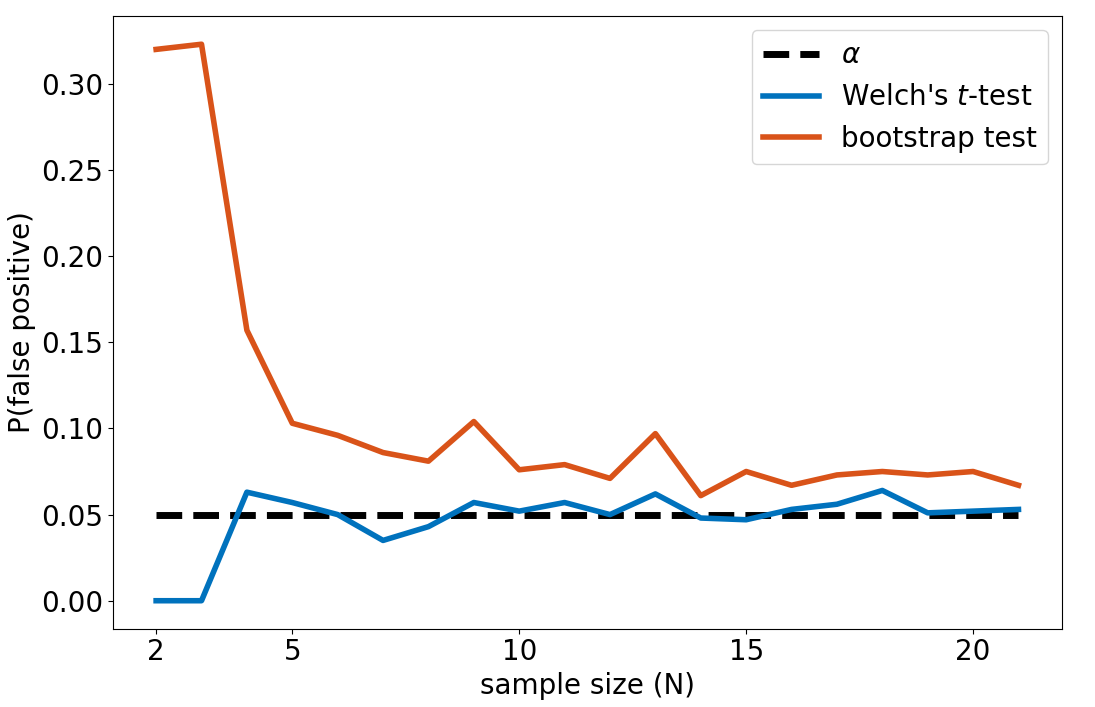
In our experiment, the bootstrap confidence interval test should not be used with small sample sizes (<10). Even in this case, the probability of type-I error (\approx10\%) is under-evaluated by the test (5\%). The Welch’s t-test controls for this effect, because the test is much harder to pass when N is small (due to the increase of t_\alpha). However, the true (empirical) false positive rate might still be slightly under-evaluated. In this case, we might want to set the significance level to \alpha<0.05 to make sure the true positive rate stays below 0.05. In the bootstrap test, the error is due to the inability of small samples to correctly represent the underlying distribution, which impairs the enforcement of the false positive rate to the significance level \alpha. Concerning the Welch’s t-test, this might be due to the non-normality of our data (whose histogram seems to reveal a bimodal distribution). In Example 1, we used N=5 and encountered a type-I error. We can see on the Figure 8 that the probability of this to happen was around 10\% for the bootstrap test and above 5\% for the Welch’s t-test.
Influence of the empirical standard deviations
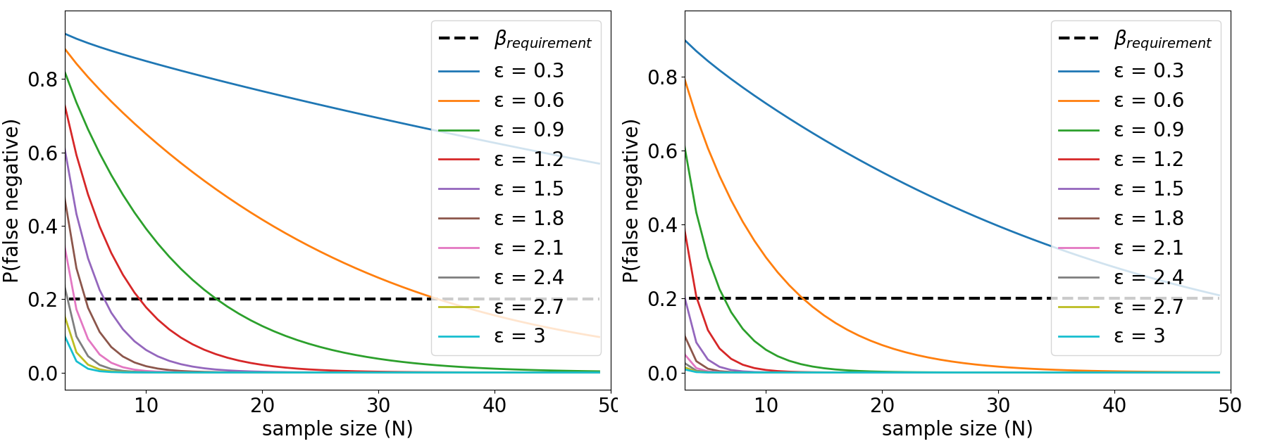
The Welch’s t-test computes t-statistics and the degree of freedom \nu based on the sample size N and the empirical estimations of standard deviations s_1 and s_2. When N is low, estimations s_1 and s_2 under-estimate the true standard deviation in average. Under-estimating (s_1,s_2) leads to smaller \nu and lower t_\alpha, which in turn leads to lower estimations of \beta. Finally, finding lower \beta leads to the selection of smaller sample size N to meet \beta requirements. We found this had a significant effect on the computation of N. Figure 9 shows \beta the false negative rate when trying to detect effects of size \epsilon between two normal distributions \mathcal{N}(3,1) and \mathcal{N}(3+\epsilon,1). The only difference between both figures is that the left one uses the true values of \sigma_1, \sigma_2 to compute \beta, whereas the right figure uses (inaccurate) empirical evaluations s_1,s_2 to compute \beta. We can see that the estimation of standard deviations influences the computation of \beta, and the subsequent choice of an appropriate sample size N to meet requirements on \beta. See our paper for further details.
Important:
- One should not blindly believe in statistical tests results. These tests are based on assumptions that are not always reasonable.
- \alpha must be empirically estimated, as the statistical tests might underestimate it, because of wrong assumptions about the underlying distributions or because of the small sample size.
- The bootstrap test evaluation of type-I error is strongly dependent on the sample size. A bootstrap test should not be used with less than 20 samples.
- The inaccuracies in the estimation of the standard deviations of the algorithms (s_1,s_2), due to small sample sizes n in the preliminary study, lead to under-estimate the sample size N required to meet requirements in type-II errors.
Conclusion
In this post, I detailed the statistical problem of comparing the performance of two RL algorithms. I defined type-I and type-II errors and proposed ad-hoc statistical tests to test for performance difference. Finally, I detailed how to pick the right number of random seeds (your sample size) so as to reach the requirements in terms of type-I and II errors and illustrated the process with a practical example.
The most important part is what came after. We challenged the hypotheses made by the Welch’s t-test and the bootstrap test and found several problems. First, we showed significant difference between empirical estimations of the false positive rate in our experiment and the theoretical values supposedly enforced by both tests. As a result, the bootstrap test should not be used with less than N=20 samples and tighter significance level should be used to enforce a reasonable false positive rate (<0.05). Second, we show that the estimation of the sample size N required to meet requirements in type-II error were strongly dependent on the accuracy of (s_1,s_2). To compensate the under-estimation of N, N should be chosen systematically larger than what the power analysis prescribes.
Final recommendations
- Use the Welch’s t-test over the bootstrap confidence interval test.
- Set the significance level of a test to lower values (\alpha<0.05) so as to make sure the probability of type-I error (empirical \alpha) keeps below 0.05.
- Correct for multiple comparisons in order to avoid the linear growth of false positive with the number of experiments.
- Use at least n=20 samples in the pilot study to compute robust estimates of the standard deviations of both algorithms.
- Use larger sample size N than the one prescribed by the power analysis. This helps compensating for potential inaccuracies in the estimations of the standard deviations of the algorithms and reduces the probability of type-II errors.
Note that I am not a statistician. If you spot any approximation or mistake in the text above, please feel free to report corrections or clarifications.
References
-
Henderson, P., Islam, R., Bachman, P., Pineau, J., Precup, D., & Meger, D. (2017). Deep Reinforcement Learning that Matters. link
-
Mnih, V.; Badia, A. P.; Mirza, M.; Graves, A.; Lillicrap, T.; Harley, T.; Silver, D.; and Kavukcuoglu, K. 2016. Asynchronous methods for deep reinforcement learning. In International Conference on Machine Learning, 1928–1937. link
-
Schulman, J.; Wolski, F.; Dhariwal, P.; Radford, A.; and Klimov, O. 2017. Proximal policy optimization algorithms. link
-
Duan, Y.; Chen, X.; Houthooft, R.; Schulman, J.; and Abbeel, P. 2016. Benchmarking deep reinforcement learning for continuous control. In Proceedings of the 33rd International Conference on Machine Learning (ICML). link
-
Gu, S.; Lillicrap, T.; Ghahramani, Z.; Turner, R. E.; Schölkopf, B.;
and Levine, S. 2017. Interpolated policy gradient: Merging on-policy and off-policy gradient estimation for deep reinforcement learning. link -
Lillicrap, T. P.; Hunt, J. J.; Pritzel, A.; Heess, N.; Erez, T.; Tassa, Y.; Silver, D.; andWierstra, D. 2015. Continuous control with deep reinforcement learning. link
-
Schulman, J.; Levine, S.; Abbeel, P.; Jordan, M.; and Moritz, P. 2015a. Trust region policy optimization. In Proceedings of the 32nd International Conference on Machine Learning (ICML). link
-
Wu, Y.; Mansimov, E.; Liao, S.; Grosse, R.; and Ba, J. 2017. Scalable trust-region method for deep reinforcement learning using kronecker-factored approximation. link
-
Plappert, M., Houthooft, R., Dhariwal, P., Sidor, S., Chen, R. Y., Chen, X., … & Andrychowicz, M. (2017). Parameter space noise for exploration. link
Code
The code is available on Github here.
Paper
Colas, C., Sigaud, O., & Oudeyer, P. Y. (2018). How many random seeds? statistical power analysis in deep reinforcement learning experiments. arXiv preprint arXiv:1806.08295 .
@article{colas2018many,
title={How many random seeds? statistical power analysis in deep reinforcement learning experiments},
author={Colas, C{'e}dric and Sigaud, Olivier and Oudeyer, Pierre-Yves},
journal={arXiv preprint arXiv:1806.08295},
year={2018}
}
Contact
Email: cedric.colas@inria.fr